Projects
I find that projects, while not constituting original research, are a fun way to familiarize myself with different fields and their contemporary and historical methods. Below you can find descriptions of a variety of projects I have completed either independently, in preface to research, or as a substantial project in a course.
2025
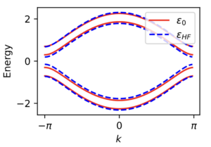
Hartree-Fock is a standard tool in the study of electronic correlations in the presence of interactions. The method decomposes four-point interactions into a product of a two-point function and a mean field expectation value of a two-point functions. This is the essence of the variational ansatz: it assumes that Wick’s theorem holds and then optimizes over states for which Wick’s theorem holds (Slater determinants). The value of the mean fields are determined self-consistently from an initial guess of their values and an iteration given the current updated values and the Hamiltonian. See the figure below for the convergence and Hartree-Fock bands (minus the Hartree shift) as detailed in my first notebook.
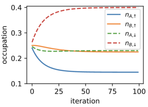
Here we consider a the Rice-Mele chain with Hubbard interaction in real space

or in momentum space the Hubbard interaction becomes non-local

but once we do the mean-field decoupling it will be local in k-space.
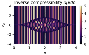
Now, the key benefit of Hartree-Fock is that it can treat large systems quickly without succumbing to the exponential scaling of exact diagonalization. This speed can be utilized to quickly calculate observables such as the (inverse) compressibility where interactions lead to incompressible states at rational fillings
the magnetization in response to an applied field
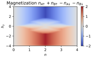
and the charge imbalance leading to charge density wave formation
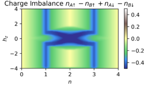
learn more in my second notebook.
Other properties can be calculated in Hartree-Fock, including the distribution of charge density in real and momentum space, topological properties such as the Berry/Zak phase and Chern number, superconducting correlations when the anomalous Bogoliubov correlators are included, and total energy of a system which enables the calculation of mean-field phase diagrams.
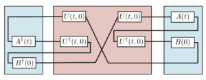
The spreading of operators that initially commute and their loss of commutativity over time is a key property of quantum dynamics and quantum chaos. To diagnose this operator spreading and non-commutativity one may consider an out-of-time-ordered-correlator (OTOC). On a classical computer one can compute the Lanczos iteration of a known Hamiltonian and the Lanczos coefficients bounds the growth rate of the OTOC (Parker et al (2019)). Meanwhile on a quantum computer one can directly model quantum dynamics and evaluate OTOCs (Google Quantum AI (2025A) and Google Quantum AI (2025B)). One may then wonder whether quantum supremacy has been achieved in these lossy/dissipative NISQ devices or whether the results are classically simulable. Talking with Martin Claassen, we came up with several expressions for calculations of OTOCs on classical computers using superoperators for open quantum systems, including one compatible with a bi-Lanczos iteration (see image above), or read more in my notes.
… coming soon …
The description of light as quanta is perhaps most appropriate when a standing wave forms as in an optical cavity. One may ask how these cavity modes (a) interface with free space modes (b) in a fully quantum-mechanical approach. The answer was provided by Collett and Gardiner, PRA 31, 3761 (1985) who found the frequency space expression for the output
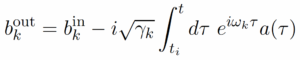
or in Fourier time-domain, the output is given by a convolution
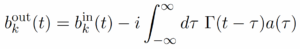
Learn more about where the input-output relation comes from and how it is derived in my notes.
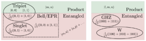
Entering in to quantum optics there are many names for different few photon states including number/Fock states, coherent states, squeezed states, thermal states, cat states, and more. In my notes I clearly list commonly (and not so commonly) encountered states and describe their decomposition into number states and the action of displacement and squeezing operators.
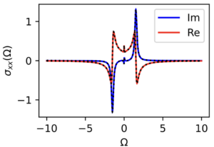
In npj Quantum Materials 9, 104 (2025), Martin Claassen and I developed a formalism for calculating observable response functions for open quantum systems. The formalism works for a broad class of systems described by quadratic Lindblad master equations, a.k.a. single particle Lindbladians; this class includes models of particles with either fermionic or bosonic exchange statistics, either with or without anomalous pairing fields (Nambu terms). In the paper we provide examples for bilayer graphene, the XY spin chain, and an optical lattice of bosons. In this project I polished the code and made it accessible on GitHub, where an example iPython notebook calculates response functions (including density, spectral function, linear and non-linear optical response) for the 1D Rice-Mele model with dissipative gain/loss processes.
2024
(Feynman) Diagrammatic techniques are a powerful perturbative method for iteratively calculating the effect of weak non-linearities on a system. For a system described by the free action S0, when a weak Kerr nonlinearity with strength K is added, to leading order in K, the partition function is modified to
![]()
which for a quantum system described by a Keldysh action with Greens functions GR, GA, and GK can be diagramatically expressed as
![]()
One can also compute modifications to the density
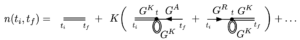
where here the leading order corrections are the Hartree diagram. Learn more in my notes.
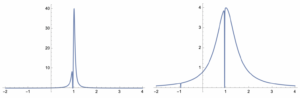
Following the 2024 Capri Spring School on Non-Unitary Many-Body Quantum Dynamics, Kilian Seibold asked me to what extent Keldysh techniques could be used for open systems with non-linearities, such as those in a Kerr-Cat qubit. One particularly straightforward approach is to take a mean field approximation where terms with four fields are broken into two field terms times a mean field density (that can be determined self-consistently). For open systems this is done in McDonald and Clerk (2023) and see my notes for a simplification of that analysis and a calculation of observables such as the spectral function (image above: left–weak dissipation, right–strong dissipation) and the density.
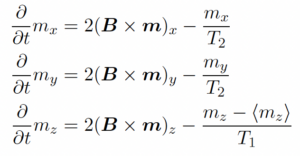
The magnetization dynamics of spins is key to both developed technologies like NMR/MRI and emerging technologies like spin qubits. In the presence of dissipation, T1 and T2 times become finite and lead to damping and a loss of coherent dynamics at long times. Following a textbook exercise I derived the magnetization dynamics of a spin coupled to a bosonic thermal bath described by a Lindblad type mater equation. Learn more and see the steps of the derivation in my notes.
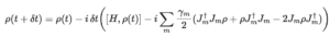
Similar to closed systems, tensor networks and TEBD can be used to simulate the time evolution of open systems. This works through vectorizing the density matrix (a matrix product operator) so that it looks like a state (a matrix product state). In this case the time-evolution is given by

which could also have been obtained through naive integration of the density matrix
Here I provide some code I have written in a Jupyter notebook to exactly simulate Lindblad dynamics for small open systems, and in another notebook provide code to simulate Lindblad dynamics using tensor networks and TEBD. While the number of sites is small in these example codes this is to benchmark the tensor network methods against the exact methods, and the tensor network methods can handle spin chains of length L = 64 with bond dimension χ = 20 in one hour without further optimization.

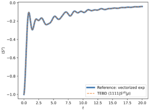
Similar to DMRG (see below), TEBD is a matrix-product state (MPS)/matrix-product operator (MPO) based tensor network algorithm. In particular, TEBD for Hamiltonians with commuting terms (for example neighbor only models partitioned into even and odd bond terms), exploits the Suzuki-Trotter expansion to time-evolve in discrete time steps without exponentiating a matrix. While this turns an initial MPS into a more complicated tensor, using SVD this can be reduced back to a MPS after each time step. Similar to DMRG, the run-time of TEBD scales polynomially in system size which means that much larger system sizes can be reached than in exact diagonalization. To implement this wrote exact diagonalization code and a class for the Heisenberg spin-1/2 XYZ model and then ran TEBD using TenPy. As visualized in the plot below, TEBD agrees quite well with exact diagonalization at short times in this system. Learn more in my Jupyter notebook.

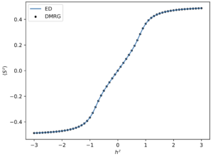
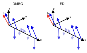
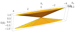
DMRG (Density Matrix Renormalization Group) is a tensor-network based approach to find the ground state of a hamiltonian. The approach fundamentally rests on discarding the high entanglement entropy sector (fixing bond dimension) with the guiding principle that ground states are typically much less entangled than excited states; this assumption means that the scaling of run time with system size is polynomial instead of exponential so that much larger system sizes (order 100 sites) can be reached. To conduct this truncation an initial trial state is constructed as a matrix product state (MPS) and then the state is iteratively optimized one bond at a time (using SVD and discarding the smallest singular values) until all bonds have been optimized. The process then repeats until convergence in the MPS is obtained. To approach this method I chose to study the 1D transverse field Ising Model and its magnetization as a function of transverse field. I wrote exact diagonalization code and a class for the Ising model and then ran DMRG using TenPy. As one can see the results of exact diagonalization and DMRG agree quite well. Learn more in my Jupyter notebook for the Ising Model. This can be extended to many other models, including the Heisenberg XYZ model where I plot the magnetization in 3D to visualize its evolution along a chain. Learn my Jupyter notebook for the XYZ Model.
2023
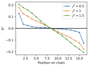
Figure: steady state magnetization in a boundary driven 16-site Heisenberg XXZ spin chain exhibiting ballistic (Jz=0.5), superdiffusive (Jz=1), and diffusive (Jz=1.5) spin transport.
The XXZ quantum spin chain is a Bethe-ansatz integrable model. Curiously at the XXX point the spin transport is KPZ superdiffusive (prediction Znidaric (2011), review by Bertini et al (2021), and claimed observation Google Quantum AI (2024)). Inspired by this, Charles Kane asked whether there could be other universality classes of anomalous transport. To answer this I found the classical set of “Fibonacci” universality classes in the literature (Popkov et al (2015)), where I rederived their results. In a followup work (Popkov and Schütz (2024)), it is argued that Onsager reciprocity forbids these other classes in the absence of additional conservation laws. The quantum case appears to be open; a 5/3 or 8/5 diffusion class would be an interesting result, perhaps achieved through spin ladders.
Inspired by the predication (Kwan et al (2021)) and observation (Nuckolls et al (2023)) of the incommensurate Kekule spiral (IKS) order in small twist angle bilayer graphene, Eugene Mele and I wondered whether a similar Kekule-type distortion could occur in large twist angle structures. In monolayer graphene the distortions have been classified an a key distortion is the sqrt(3) x sqrt(3) unit cell tripling distortion (Chamon et al (2012))
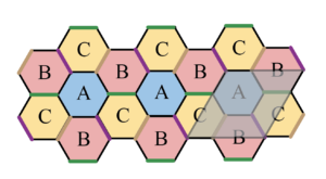
While we found phase windings with larger unit cells in commensurate bilayers than in the monolayer, we concluded that the IKS order is fundamentally driven by interactions that need to be accounted for at a Hartree-Fock level at a minimum and that interactions in the dispersive bands at large twist angles might be irrelevant. See my slides and my other slides for more.
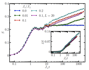
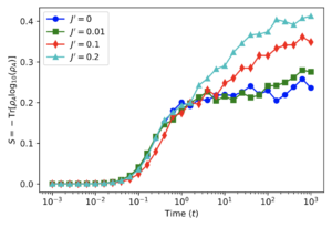
The von Neumann entanglement entropy for bipartitions of a chain can provide valuable information on the structure of the quantum states present. In particular how the entanglement entropy scales with system size and the length of the bipartition, e.g. constant, logarithmic, or linear, can provide insight into the level of entanglement, and hence quantities such as the thermalization of the system. To study this, I followed the work of Bardarson, Pollmann, and Moore in Phys. Rev. Lett. 109, 017202 (2012) to investigate the scrambling of initially unentangled product states under time evolution. Here a random initial product state is time-evolved using the XXZ hamiltonian with Z magnitude J’. The results show a rapid initial onset of entanglement followed by a plateau, and a subsequent long-time linear increase in the entanglement entropy. Learn more in my Jupyter notebook.
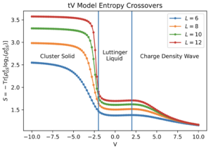
In addition to quantifying the dynamics of quantum systems, the entanglement entropy can be used to quantify the ground states of quantum systems. Following the work of Barghathi et al in Phys. Rev A 100, 022324 (2019), I investigated the ground state entanglement of the fermionic tV model (nearest neighbor hopping strength t and nearest neighbor density-density interaction V) which exhibits three phases as a function of interaction strength. These ground states have distinct orders that are captured by the entanglement entropy. Learn more in my Jupyter notebook for the entanglement crossover. Additionally, by studying how the entanglement entropy varies with bipartition size, one can extract the central charge of an effective field theory in the manner of Cardy and Calabrese J. Stat. Mech. 406, P06002 (2004) and Refeal and Moore Phys. Rev. Lett. 93, 260602 (2004). Learn more in my Jupyter notebook for the central charge.
 .
. 
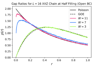
Long term storage of quantum information is a crucial for the development of quantum computing technologies. In non-interacting systems quantum interference due to disorder can lead to localization. It is natural to ask whether a strongly interacting, many-body system can localize information at long times as well. Generically one expects any arbitrarily small integrability breaking terms to result in thermalization and a diffusion of information to inaccessible non-local degrees of freedom. But can one localize this information even if such integrability breaking terms are present? The postulated many-body localized phase claims to do this. Here I study use exact diagonalization to study the level statistics which measure localization. Learn more in my report.

d orbitals can hold up to ten electrons, and while in free space the energy of the orbitals are all the same, in a molecule or a crystal the “crystal field” leads to a splitting between high energy and low energy orbitals. The combined system is then governed by a Hamiltonian involving the Coulomb repulsion of the electrons and the crystal field. The optical properties of the compound will then depend on the strength of the crystal splitting Dq. A plot of the many-body energies as a function of the crystal field splitting is known as a Tanabe-Sugano diagram: see the figure below for one with four electrons. Here I use exact diagonalization to study the many-body energies of these structures and observe the high-spin to low-spin transition in the d4 transition metal complexes at critical field Dq=2.6683B. See the steps in my Jupyter notebook.

Python is a high level programming language with a reputation for slow runtimes. To overcome this there are a variety of approaches including pre-compiling functions and caching previous data. Another approach that is built in to NumPy and one that is particularly applicable to physics problem is the Einsum function. Einsum performs tensor operations (contractions, matrix multiplications, traces, etc) naturally and quickly with a huge speedup over naive implementations. Here I demonstrate the use of Einsum for the Kubo formula calculation of optical conductivity in a two-band model. This example illustrates a variety of Einsum functionalities including how to use Einsum to sum over reciprocals and how to broadcast using the None routine. Learn more in my Jupyter notebook.

2022
For systems in equilibrium, expectation values for observables can be obtained by evaluating the observable on an open time-evolution contour from large negative times to large positive times. However this equilibrium scenario is not generic, and the calculation is only enabled by the fact that the total time evolution constitutes a total phase which can be absorbed into the definition of the many-body wavefunction. Generically quantum systems need not be in equilibrium, and a time evolution need not bring the state back to itself (up to a phase), and expectation values for observables must be evaluated on closed time-evolution contours. This is the Keldysh contour, and from it under a change of basis one finds the Keldysh Greens function which gives the correlations between the advanced and retarded Greens functions. Learn more in my notes.

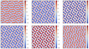
Intense illumination can both qualitatively and quantitatively alter the electronic behavior of materials. This was unequivocally shown by Kogar et al in Nat. Phys. 16, 159 (2020), where illumination of charge density wave material LaTe3 changed the charge density wave order from smectic to a crystalline checkerboard order. Phenomenologically this can be explained by rescaling parameters in the Landau free energy enabling the coexistence of charge density wave orders in two directions. Microscopically this behavior can be explained by the light driving a gap in the Fermi surface to close again after it had been opened by the formation of the first charge density wave order. Here I discuss this work in the context of liquid crystals; learn more in my notes.

Fig. Illuminating LaTe3 with light fundamentally alters its charge density wave order structure.
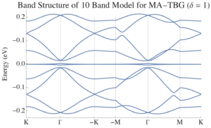
Magic-angle twisted bilayer graphene exhibits flat bands near the Fermi energy. There are many ways to model the electronic structure of this material, such as the tight-binding model of the tab below this one, but many of these models consider far more bands than are relevant to describe the low energy physics of the system. A recent thread in the construction of effective models for systems is to construct models with the minimum number of bands that get the band representations correct from the point groups at high symmetries. This thread was initially proposed by Bradlyn et al in Nature 547, 298 (2017), and has since been used both in the construction of low energy models and to triage materials databases for topological materials. In PRB 99, 195455 (2019), Po et al apply this methodology to obtain “faithful” models for magic-angle twisted bilayer graphene that respect the band representations and point group symmetries of this material and present its fragile topology. In a Mathematica notebook I recreated this model and plotted its band structure.
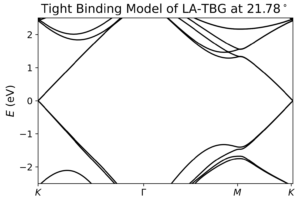
Tight-binding models are ubiquitous in solid state and molecular physics for their computational simplicity and theoretical tractability. Here I describe the tight-binding model from Nano. Lett 10, 804 (2010), in which the authors were one of the first to appreciate the flat band condition in small twist angle bilayer graphene. This was later reproduced and understood through the Bistritzer-MacDonald model (PNAS 108, 12233 (2011)) with the dispersion of the flat bands arising from slight chiral symmetry breaking terms. This Learn more about the tight-binding model parameters and see some examples in my notes.
Fractons are quasiparticles with fractionalized motion: while they may live on a lattice in D dimensions, their motion is constrained to some subset, often of lower dimensionality, that the whole lattice. The paradigmatic example of this is the X-cube model (PRB 92, 235136 (2015)), but what many fracton models have in common is that they are constrained to lattices. Now, one may seek to describe the behavior of fractons in the continuum, but this leads to conflicts with the accepted wisdom of continuum theories that all field variables should be continuous: if they are not, then Taylor expansion fails and UV divergences emerge. However, this may be avoided if there are a finite number of discontinuities in the field variables. This is the work of Seiberg and Shao (arXiv:2003.10366 (2020)), and finds that by relaxing this assumption in continuum field theory one may obtain fractonic behavior and unusual ground state degeneracies through imposing unusual global symmetries such as multipole conservation. Learn more in my slides.

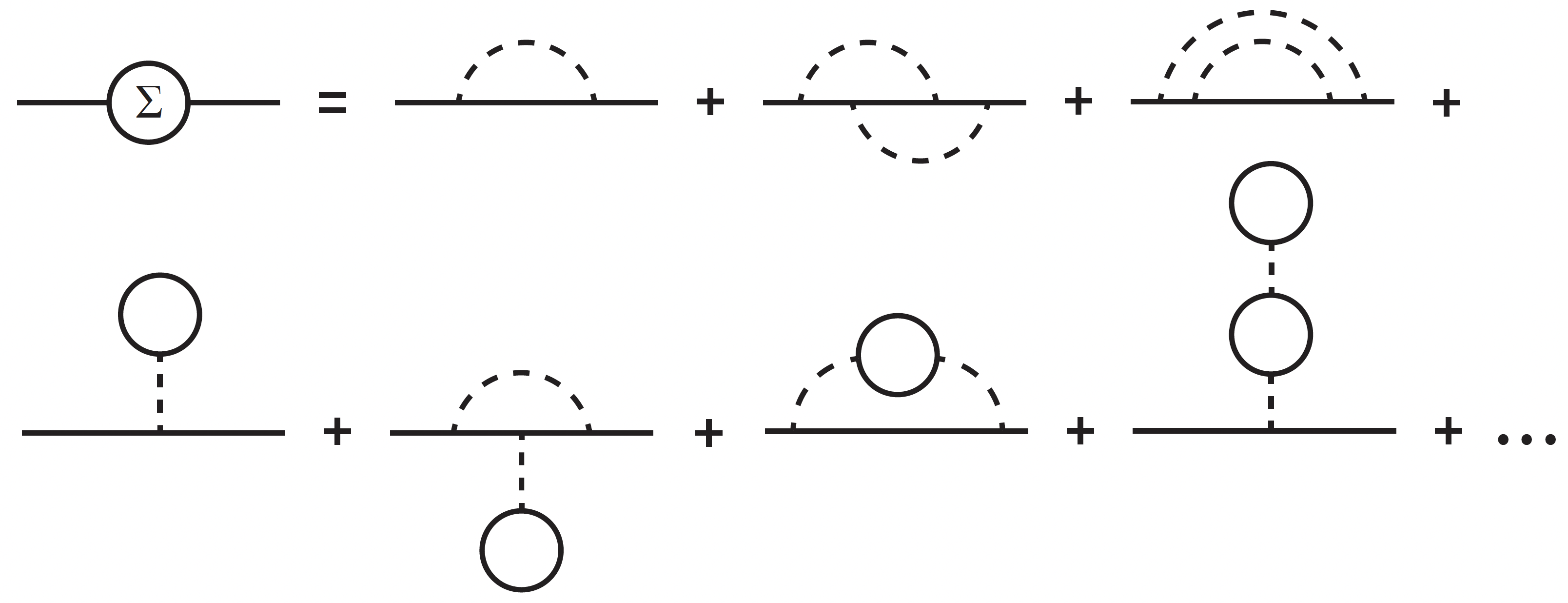
The self energy is a key concept in quantum field theory. In electronic systems it enters in the expression for dressed propagators which correspond to quasiparticle excitations in the system. Quasiparticles are inherently unstable and the imaginary part of the self energy gives the lifetime of the quasiparticle. Learn more in my notes.
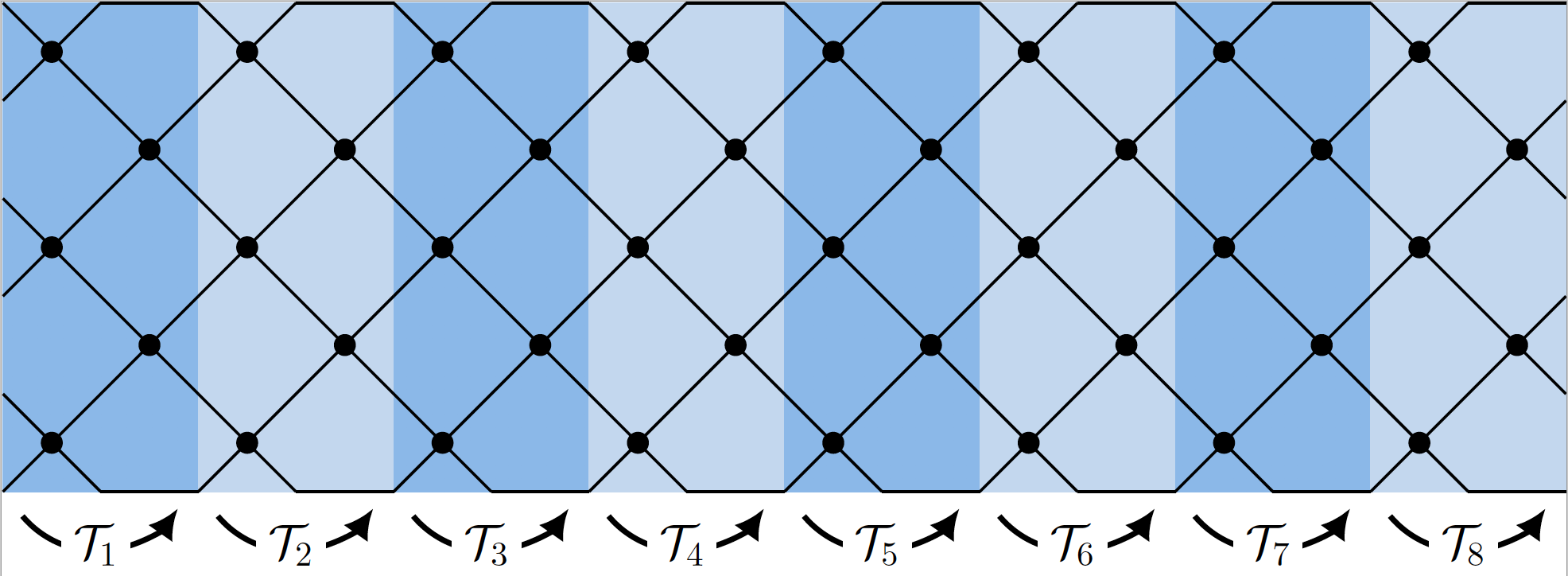
Key features of classical electromagnetism including the Maxwellian action, Gauss’s law, the energy density, and charge quantization can be derived from Abelian lattice gauge theories, e.g. theories describing spins on a lattice. In particular, many Lagrangians reduce to the same quadratic Lagrangian of electromagnetism in the long-range (small curl) limit, of which four are illustrated below. Additionally such lattice gauge theories enable the quantization of charge to be derived from the compactness of the gauge group (rather than from the presumed existence of a Dirac monopole.) Learn more in my lecture notes.
2021
Many features of the fractional quantum Hall effect including fractionalized charge and fractionalized conductance can be understood the result of a coupling between an emergent “quasiparticle” gauge field and the real electromagnetic gauge field. In particular, it is sufficient to assume that we are interested in the long-range physics of a (rotationally symmetric) system with a gap above the ground state(s). In this case we only want the lowest powers of the gauge field(s) and their derivatives, and enforcing gauge invariance on the Chern-Simons term (one gauge field and one gauge field derivative antisymmetrized by the Levi-Civita tensor) leads to a quantized and fractionally quantized Hall response. Learn more in my pedagogical introduction to the subject.
The quantum geometry—the Berry connection and the Fubini-Study metric—of Bloch states plays a central role in the stability of fractionalized states (Roy PRB 90, 165139 (2014), and Lee, Claassen, Thomale PRB 96, 165150 (2017)), present a conceptually unified picture of optical transitions (Ahn, Guo, Nagaosa, and Vishwanath (2021)), and contribute to a variety of other phenomena.
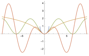
Here I follow Srivastava and Imamoglu in PRL 115, 166802 (2015) where they considered the effect of the quantum geometry of the intra-band overlap of Bloch states on exciton energies in TMDs. I extend the expansion of the intra-band overlap of Bloch states in terms of the Berry connection and the Fubini-Study metric to third and fourth order. This expansion holds for general Bloch states. I find an an additional second order term (blue) that was not obtained in the PRL paper
![]()
Learn more in my notes.
Circular dichroism is a powerful tool used to probe the symmetries of electronic states in materials, and is the phenomena responsible for making circular light polarizers possible. In a crystal with mirror symmetry, circular dichroism is non-zero only when time-reversal symmetry is broken. In finite-layer systems, circular dichroism can be used as a probe of inversion symmetry since it vanishes for inversion-symmetric systems.
As I show in these notes, once you have a momentum space Hamiltonian, calculating the circular dichroism (if any) is a straightforward procedure.

In classical mechanics, the current I through a cross-section of area A, with charge density ρ moving at velocity v is I=Aρv. Following this one can define the quantum mechanical current operator for a single electron as j=ev. One can also arrive at this from the perspective of Noether’s conserved currents, but here we use the classical-mechanical intuition. Now, for a non-relativistic electron, the velocity operator will be the gradient of the Hamiltonian with respect to the momenta. At first glance there is no issue evaluating this provided the Hamiltonian is an explicit function of momenta. However the evaluation is not necessarily so simple since the components of the gradient are expressed in the contravariant basis, while measurements of current are taken in the covariant basis. For systems with rotational symmetry (ex. a Dirac cone), or systems with orthogonal axes these bases are the same, but in general they are different. In these notes, I derive general expressions for the non-relativistic current operators for an electron on a triclinic lattice.

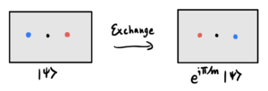
The optical absorption of a circular Dirac cone is frequency and polarization independent independent with a quantized absorbance of πα where α~1/137 is the fine-structure constant. As I show in these notes, another theoretically tractable limit is that of an elliptical Dirac cone where the Fermi velocities in the two principal directions are not (necessarily) equal. If one Fermi velocity is 100 times the other (a quasi-one-dimensional limit) then the absorbance in one direction will be 10πα and πα/10 in the perpendicular direction. In a monolayer system 10πα~23% is a massive response.
A physically relevant example of an elliptic Dirac cone occurs in the (100) surface states of the topological insulators α-Bi4I4 and β-Bi4I4 where the Fermi velocities for the two principal directions differ by factors of 74 and 14 respectively for these two materials. This means that these surface states are expected to absorb 8.63πα and 3.76πα respectively along the strand direction. Here is a schematic of the elliptic Dirac cone in β-Bi4I4
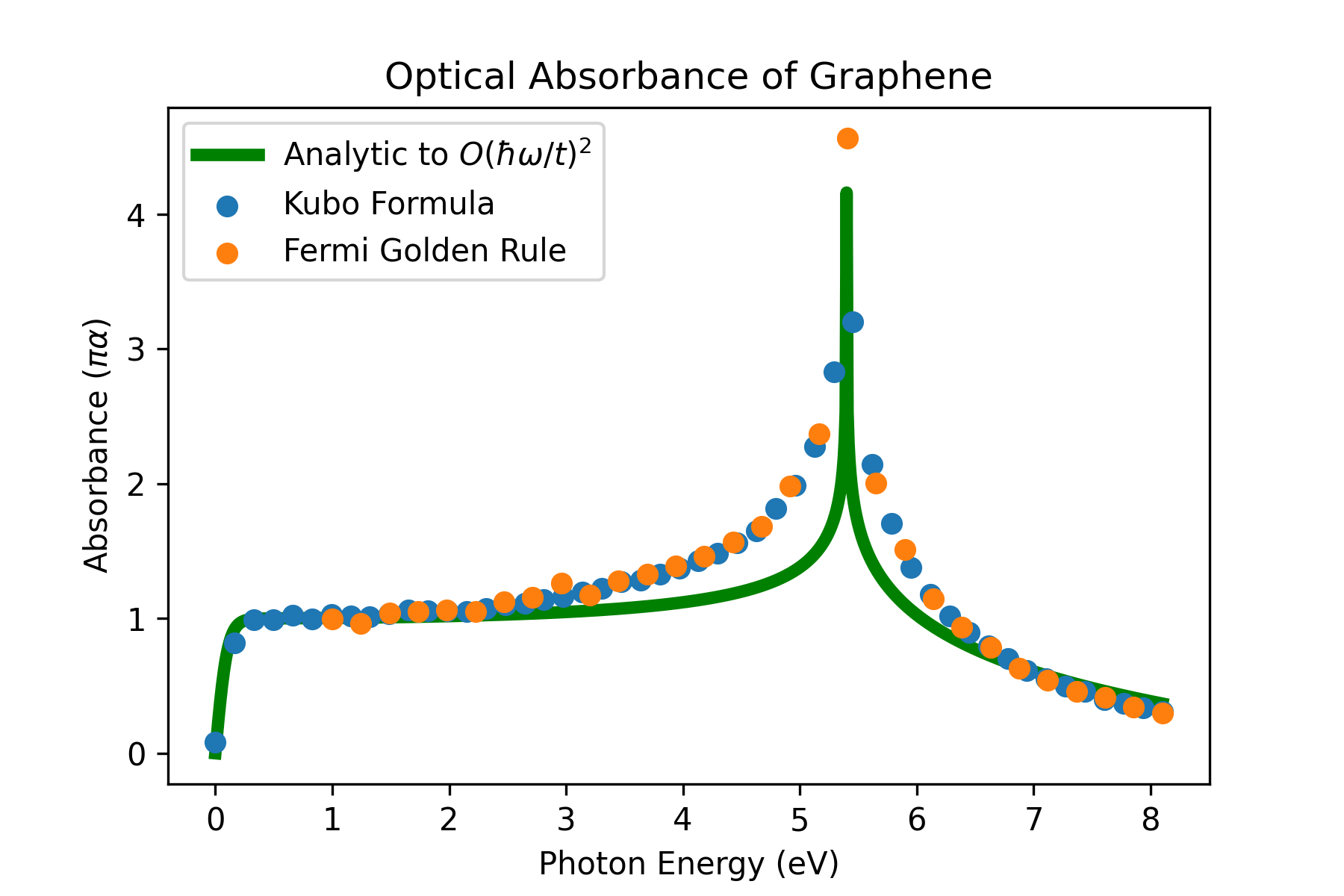
In the Dirac Cone Limit, graphene has a linear dispersion at the Fermi energy. A short derivation shows that this leads to a quantized optical absorbace of πα where α~1/137 is the fine-structure constant. However, graphene’s linear dispersion is an approximation that is most accurate at low photon energies. For higher energies, a more sophisticated analysis is necessary. Using both Fermi’s Golden Rule and the Kubo Formula, I calculated the optical absorbance of graphene in the tight-binding approximation, and compared the results to the second order analytic results by Stauber, et al.
The reference is Stauber, Peres and Geim Phys. Rev. B 78, 085432, (2008).
The less time you spend on activities like formatting your bibliography, the more time you can spend on research. Here is a guide I put together to aid this goal that includes a minimal working example of a RevTeX file with a BibTeX bibliography, guidance on how to ensure RevTeX formats your citations properly, and tips on arXiv and the submission process.
2020
The density of states in a system is fundamental to all momentum-integrated responses. While in some cases the density of states can be determined analytically, in general the density of states must be determined numerically. Here I outline a simple numerical procedure known as the “Histogram Method” to compute the density of states.
The units of the resulting density of states are 1/(energy * length^dim) where the units of energy and length (unit cell dimensions) are specified by the problem. Learn more and read about this method in my notes.
Here is the density of states for graphene, computed using this method, where t = 2.7 eV is the nearest-neighbor hopping strength

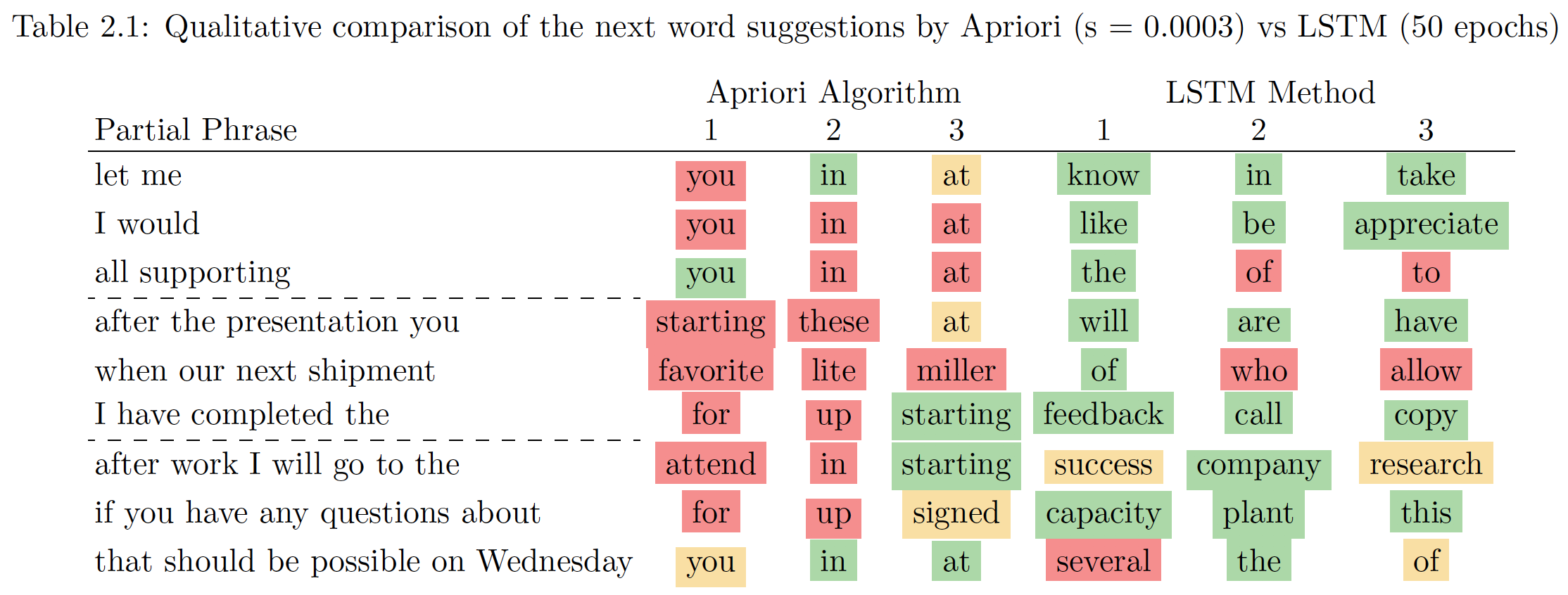
Autocomplete is a feature that predicts the rest of a word, phrase, or sentence inputted by a user. This technology is commonly available on a variety of platforms from composing texts and emails to completing search phrases. Working with fellow UCLA student Kalsuda Lapborisuth, we implemented two autocomplete methods based on the Apriori Algorithm and Long Short Term Recursive Neural Networks. To train the models we used the Enron email dataset, and qualitatively tested the methods on business-like phrases. Here is our report on these methods and our results.
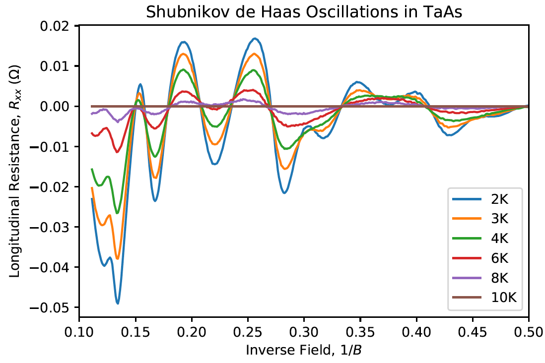
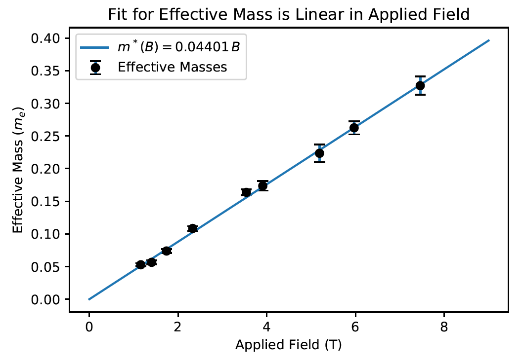
Properties that are dependent on the density of states will oscillate when the density of states oscillates. In a strong magnetic field, electrons undergo cyclotron motion and form uniformly spaced Landau Levels where the Landau Level energies depends linearly on magnetic field strength. The density of states is high at the level centers and low in between levels. One property that depends on the density of states is the resistivity, so as the magnetic field is varied, Landau Levels pass through the Fermi surface resulting in an oscillation of the resistivity known as Shubnikov de Haas Oscillations. Much information about the structure and behavior of a material can be deduced from such transport measurements.
Working with Madeline Gullen, Joshua Lee, and Eve Emmanouilidou, we performed transport measurements on single crystalline TaAs and observed the Shubnikov de Haas Oscillations. Analyzing the results we were able to conclude that TaAs is a Weyl Semimetal: it exhibits chiral anomaly, behaviors consistent with a linear dispersion, and it has a Berry phase of π. Here is my report on this experiment and our results.
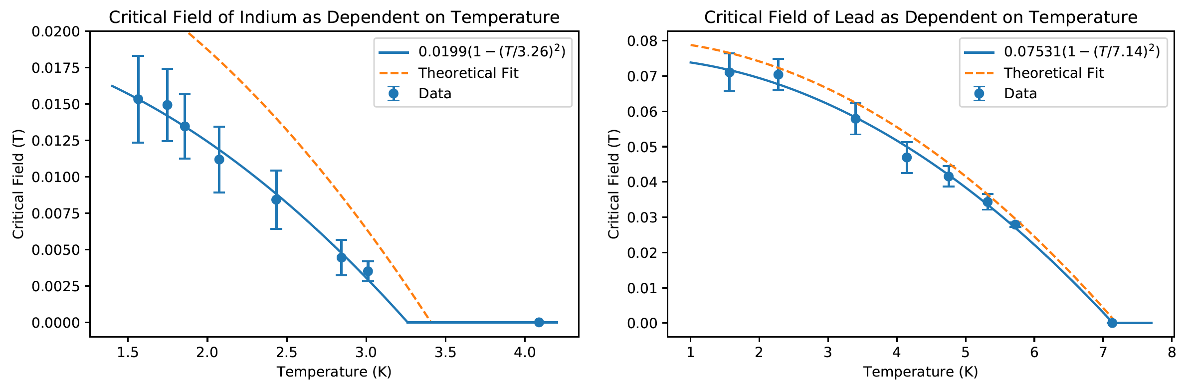
In an s-wave superconductor, L=0, and the spins of Cooper paired electrons anti-align forming a singlet state (spin-zero boson). The application of a sufficiently strong magnetic field can make spin alignment with the field energetically favorable versus Cooper pair anti-alignment, and so an applied magnetic field can induce a transition from a superconducting to normal state. The strength of the magnetic field where this happens is known as the critical magnetic field and it varies with temperature.
Working with Madeline Gullen, Joshua Lee, and Teresa Le, we performed measurements of the critical field of Indium and Lead as a function of temperature. Here is my report on this experiment and our results.
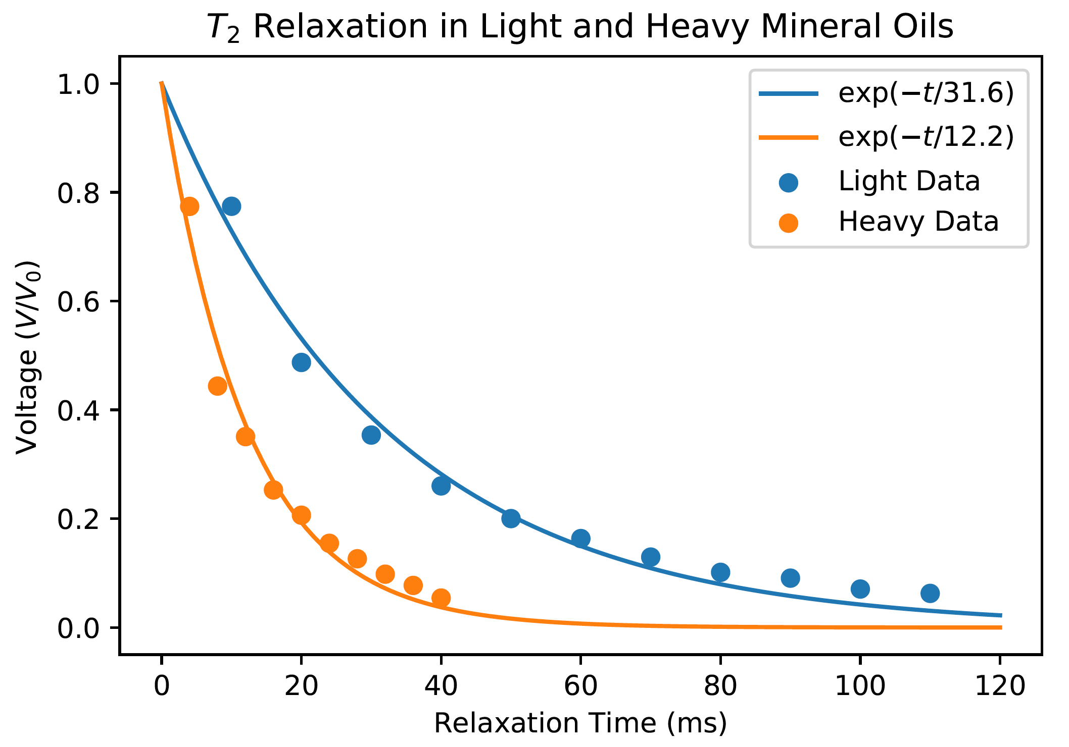
While Larmor precession and Rabi oscillations describe basic spin behaviors, they do not account for relaxation, and relaxation times can be used to characterize materials. In particular, the different spin relaxation times of different media is used in NMR Magnetic Resonance Imaging for medical applications. Working with Madeline Gullen, Joshua Lee, and Teresa Le, we observed that different media: light mineral oil, heavy mineral oil, and water all have different spin relaxation times, and that the presence of magnetic impurities such as Cu2SO4 has substantial impacts on the spin relaxation times. Here is my report on this experiment and our results.
BaTiO3 is an crystal often used as a dielectric in capacitors since it has a large dielectric constant across a wide range of temperatures. Cooling through 120C, BaTiO3 changes from a cubic to a tetragonal crystal structure. This transition mirrors the paramagnetic-to-ferromagnetic transition at the Curie temeperature, except the paraelectric-to-ferroelectic transition is a first-order phase transition.
This phase transition can be observed by determining the dielectric constant of BaTiO3 as a function of temperature. One way to do this is to use BaTiO3 as the dielectric in a capacitor, create a resonant circuit and measure the phase angle. Working with Madeline Gullen, Joshua Lee, and Teresa Le, we created a capacitor from a BaTiO3 single crystal and performed measurements of the phase angle as a function of temperature. With this method, we observed a sharp transition in the dielectric constant at 119.4C. Here is my report on this experiment and our results.

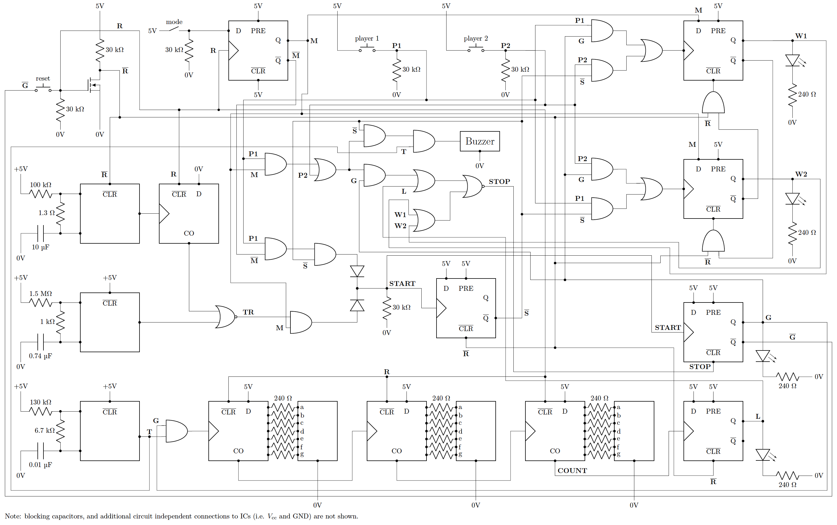
Working with fellow UCLA student Stephen Randolph, I designed, built, and documented the construction of a reaction-time game from linear circuit components, diodes, basic logic gates, flip-flops, counters, and a 555 timer. The game starts when a referee presses the start button, and at a random time between zero and five seconds after the referee’s press, a LED turns on. The first player to press their button following the LED turning on wins, and is indicated by an LED and their time on 7-segment displays. If a player false starts, a buzzer plays and the penalized player is indicated by an LED. The game can be reset by flipping a switch. The circuit design is illustrated below.
2019
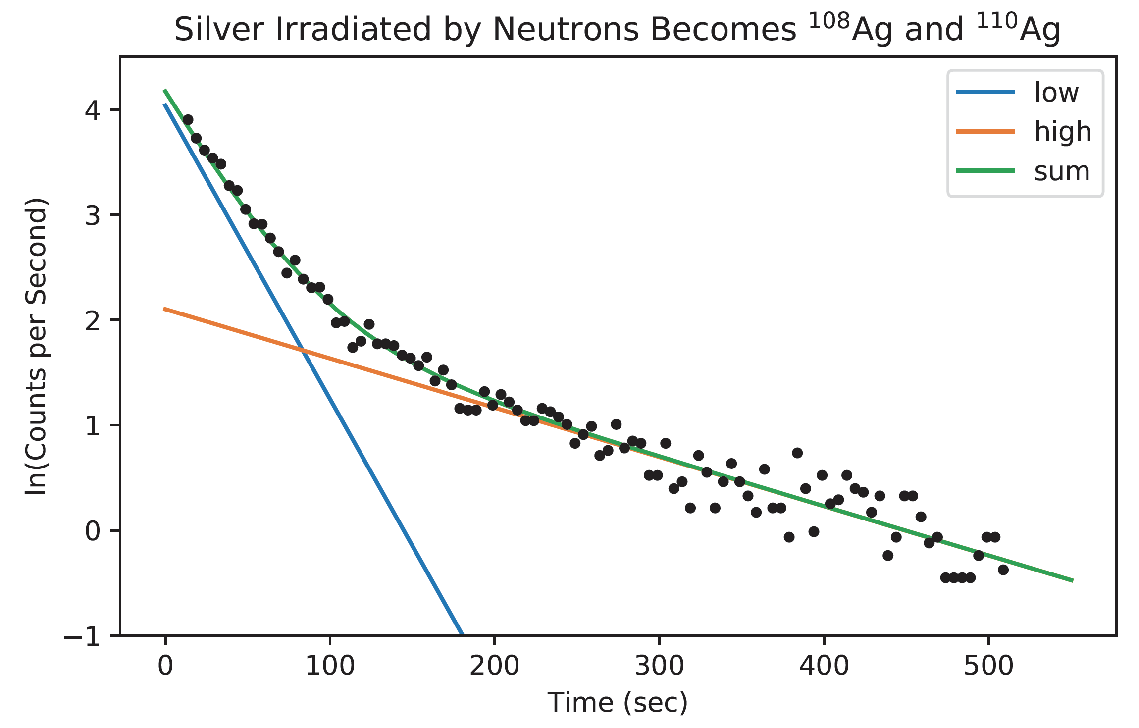
Naturally occurring silver is roughly evenly distributed between the stable isotopes Ag-107 and Ag-109. Upon absorbing a neutron Ag-107 becomes Ag-108 which has a half-life of 142 seconds, and Ag-109 becomes Ag-110 with a half-life of 25 seconds. Working with fellow UCLA student Jinghong Yang we measured the background rate of radiation, and then under the supervision of Professor Nathan Whitehorn, we irradiated silver foil samples using a 5 curie Americium-Beryllium neutron source, and measured the beta decays of the samples. Fitting for short-lifetime and long-lifetime decays, we determined a half-life of 148 seconds for one silver isotope and 25 seconds for the other silver isotope.
In a regular polygon of fixed point charges of equal magnitude, the electric field cancels at the center of the polygon. However, this is not the only place where the field cancels. In particular, there are saddle points of the scalar potential located approximately at the center of each edge of the polygon.
I determined the location of these points numerically, and a report on these studies may be found here.

Molecular dynamics simulations seek to develop an understanding of the interactions of atoms and molecules through computationally modeling interactions and evolutions. A basic application of these methods is to the behavior of a monatomic gas.
The behavior of the gas may be modeled as hard spheres that scatter elastically, conserving energy and momentum. I implemented this for particles in a square box, and colored particles according to their kinetic energies.

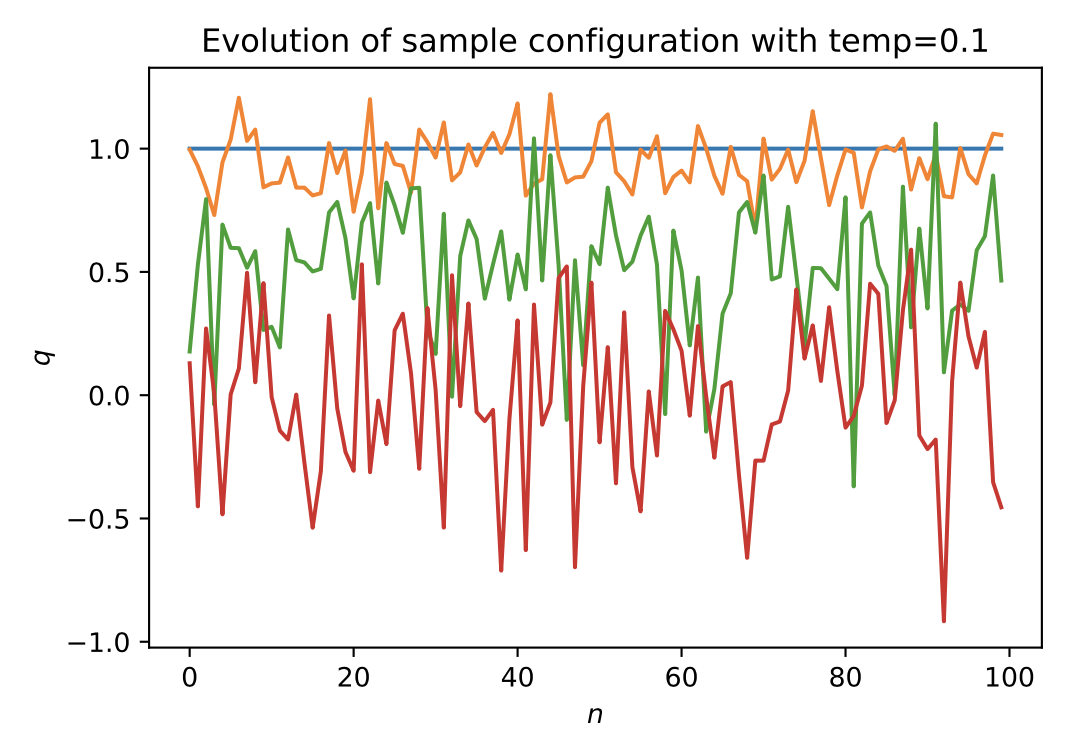
Path Integral Monte Carlo is a numerical method to approximate thermodynamic quantities for quantum systems. In particular, it is useful to investigate the behavior of systems at finite temperature where exact solutions rarely exist. Here, I developed code to implement Path Integral Monte Carlo for a given Lagrangian for a system and return the expectation values and expectation values squared of each variable. The algorithm implemented starts at high temperature and gradually cools to the desired temperature.
Here are the results of applying the Path Integral Monte Carlo to the Simple Harmonic Oscillator (a Bosonic system), where there is an exact form for the internal energy is known. On the left, configurations as a function of time are plotted for four configurations as the system cools; on the right is a comparison of the analytic and numeric results:

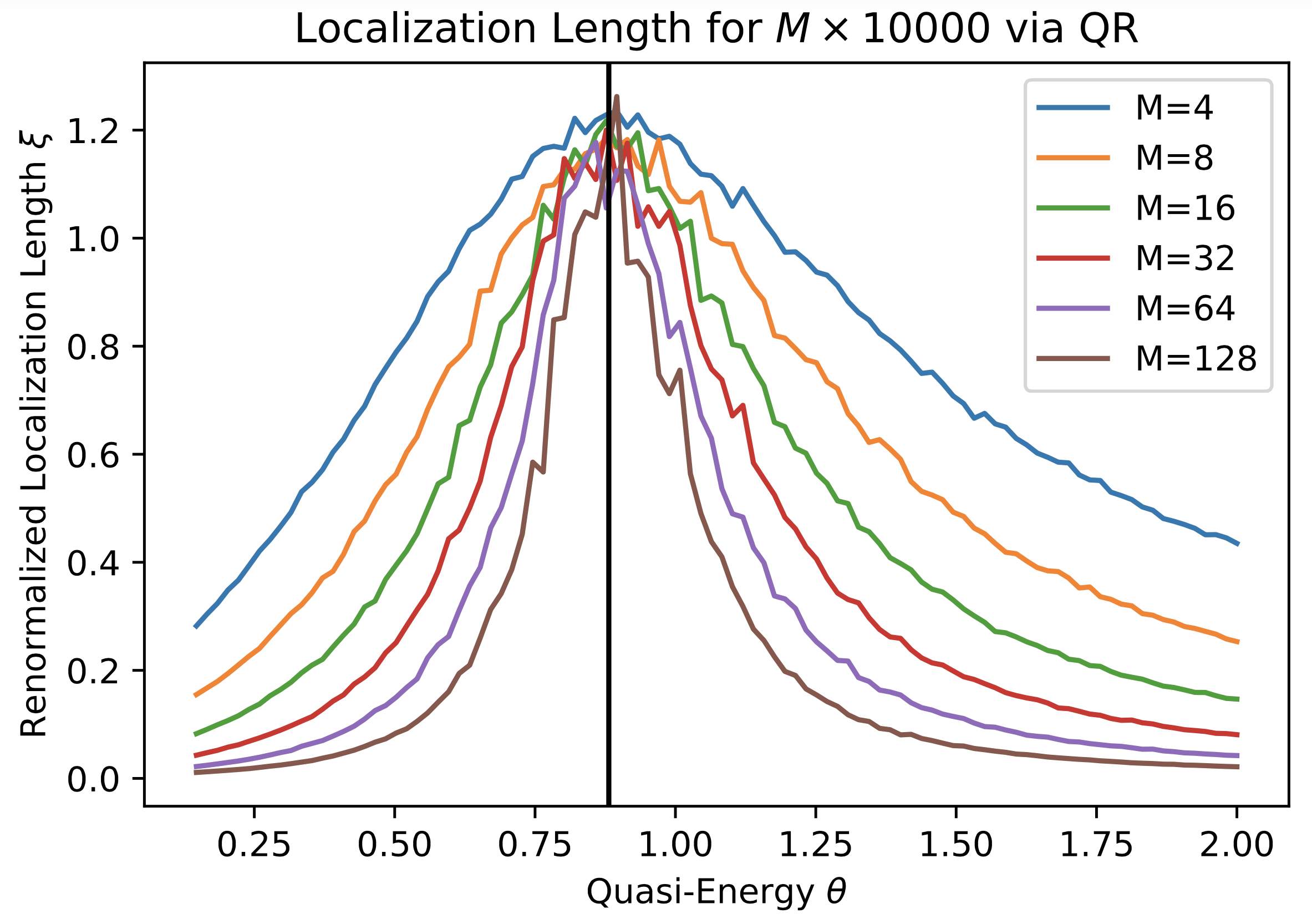
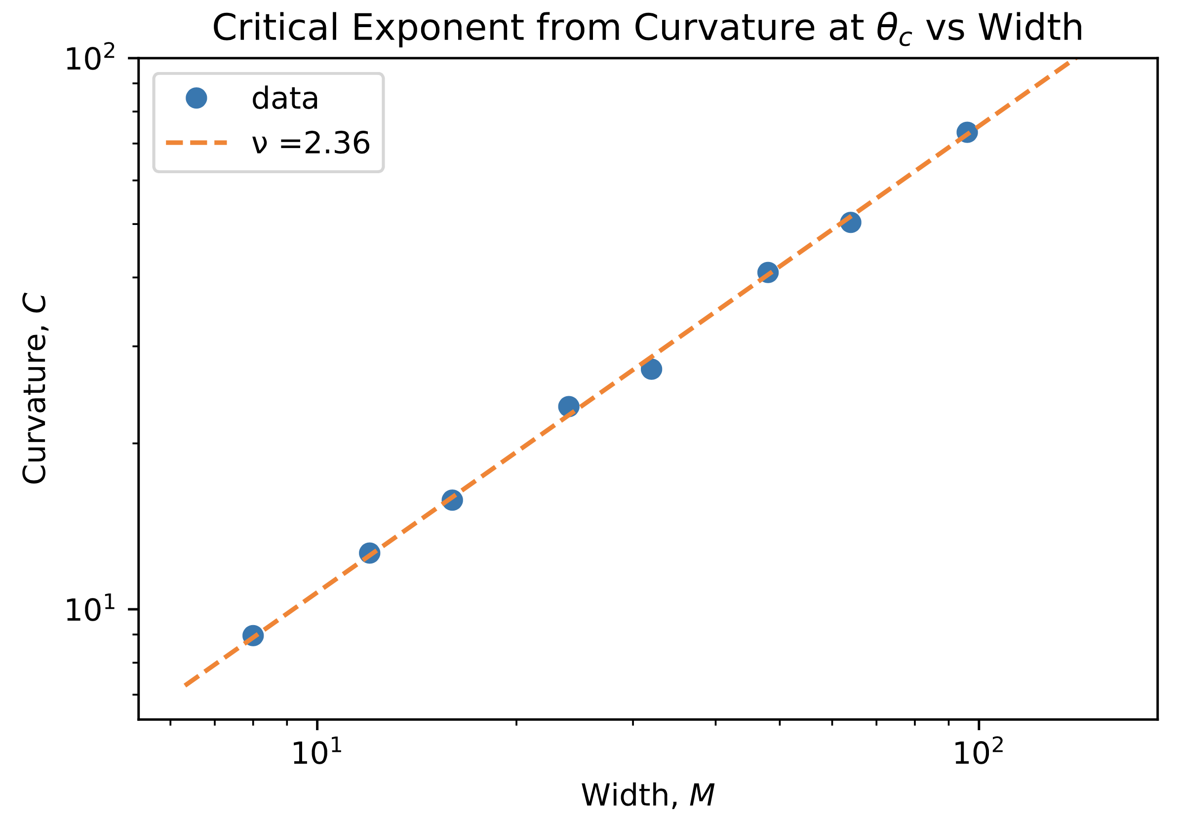
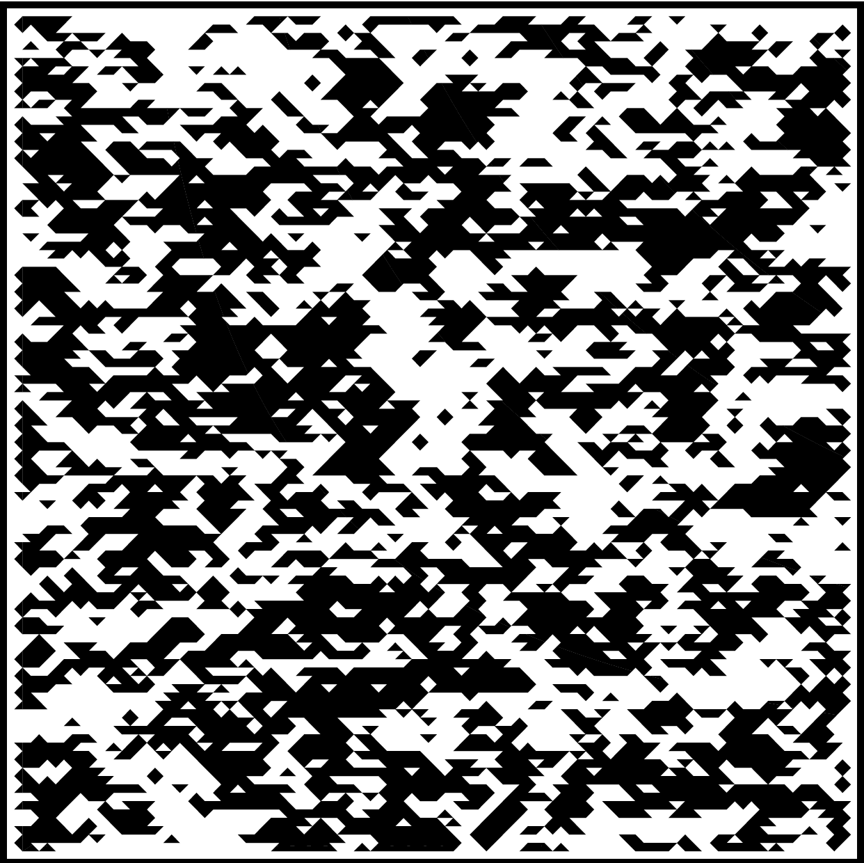
Following MacKinnon and Kramer, I developed Python code to calculate the renormalized localization length for a given set of transfer matrices. Following Chalker and Coddington, I applied this code to calculate the critical exponent for the Plateau Transition in the Integer Quantum Hall Effect. Above: the Chalker-Coddington strip. Left: localization length is linear in width M at the critical energy, θ=0.88. Right: the critical exponent is around 2.36.
The references are MacKinnon and Kramer, Z. Phys. B 53, 1 (1983) and J.T. Chalker and P.D. Coddington, J. Phys. C 21, 2665 (1988).

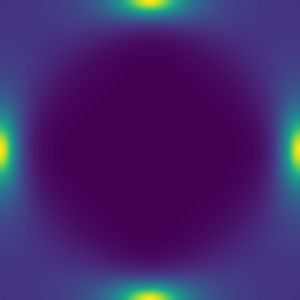
Following Fukui, et al., I developed Python code to calculate the Chern Number of a given energy band in a specified tight binding model. Above left: an energy band in the Qi-Wu-Zhang Model. Above right: its Berry Curvature. The Chern Number is 1.
The reference is T. Fukui, Y. Hatsugai, and H. Suzuki, J. Phys. Soc. Jpn. 74, 1674 (2005).
2018

I developed Python code to numerically calculate the dispersion relations for tight-binding models. Following Hofstadter, I applied this to the Harper-Hofstadter Hamiltonian and found the Hofstadter Butterfly.
The reference is D.R. Hofstadter, Phys. Rev. B 14, 2239 (1976)
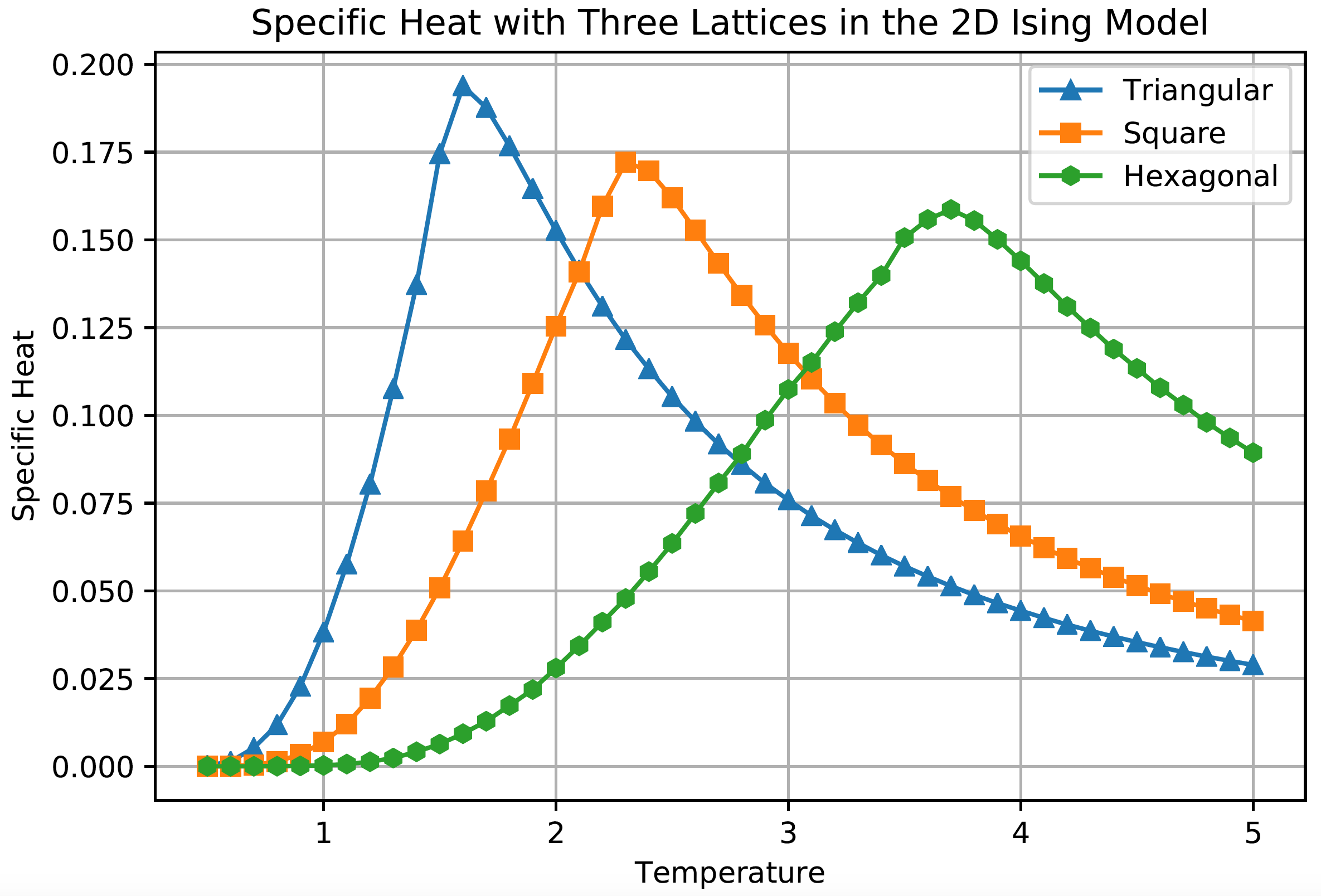
The Ising Model of ferromagnetism, or spin alignment with temperature, is a representative system for many phenomena in statistical mechanics. The two-dimensional Ising Model may be solved analytically for the square lattice as in the work of Onsager, but other geometries may only be solved numerically. I developed code to simulate the two dimensional Ising Model for triangular, square, and hexagonal lattices. The numerical results for the square lattice agreed with the Onsager’s analytic results.
Here are spin configurations on 100×100 lattices, and plots of the specific heats and magnetic susceptibilities by lattice:


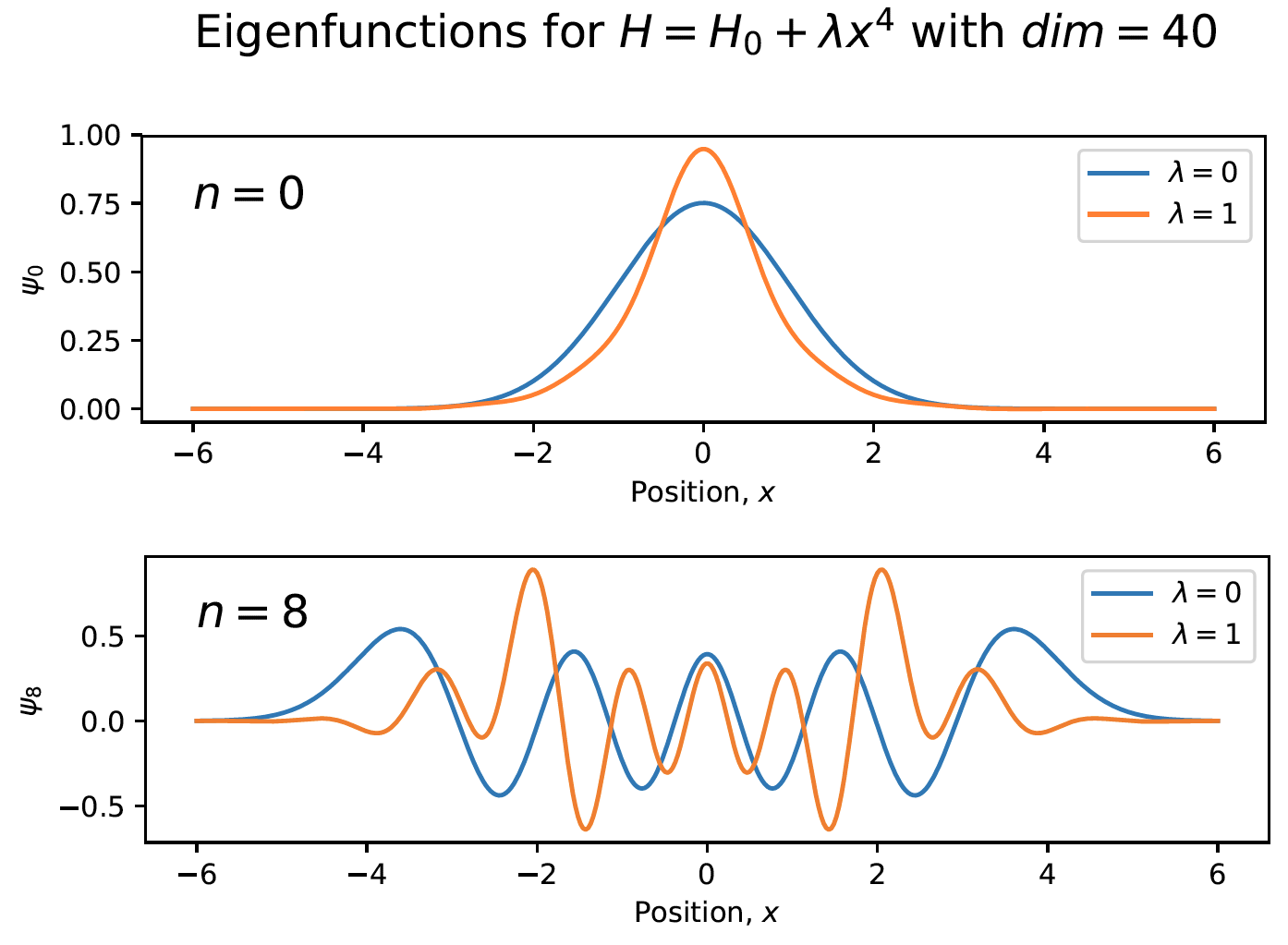
The eigenfunctions for most quantum systems cannot be determined analytically. An approximate solution to this problem is to write an approximation to the Hamiltonian matrix, and then find its eigenvectors. For some perturbations, such as a quartic perturbation to a quantum harmonic oscillator, the approximate Hamiltonian is simple to write. I developed code to write these Hamiltonian matrices in any matrix dimension, numerically diagonalized the matrices, found their eigenvectors, and converted them into real-space wave functions.
Here are plots of eigenfunctions for unperturbed and perturbed harmonic oscillators:
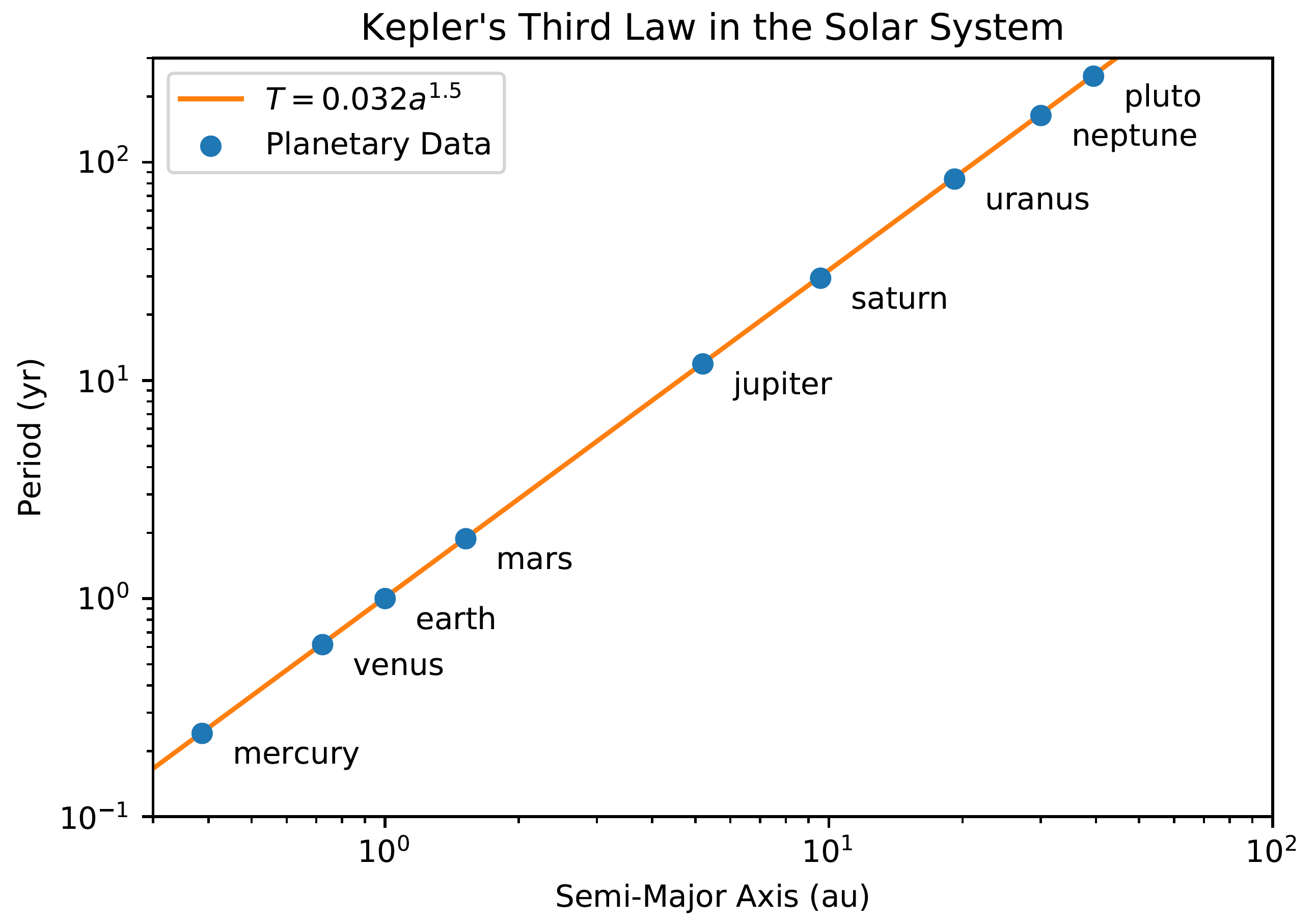
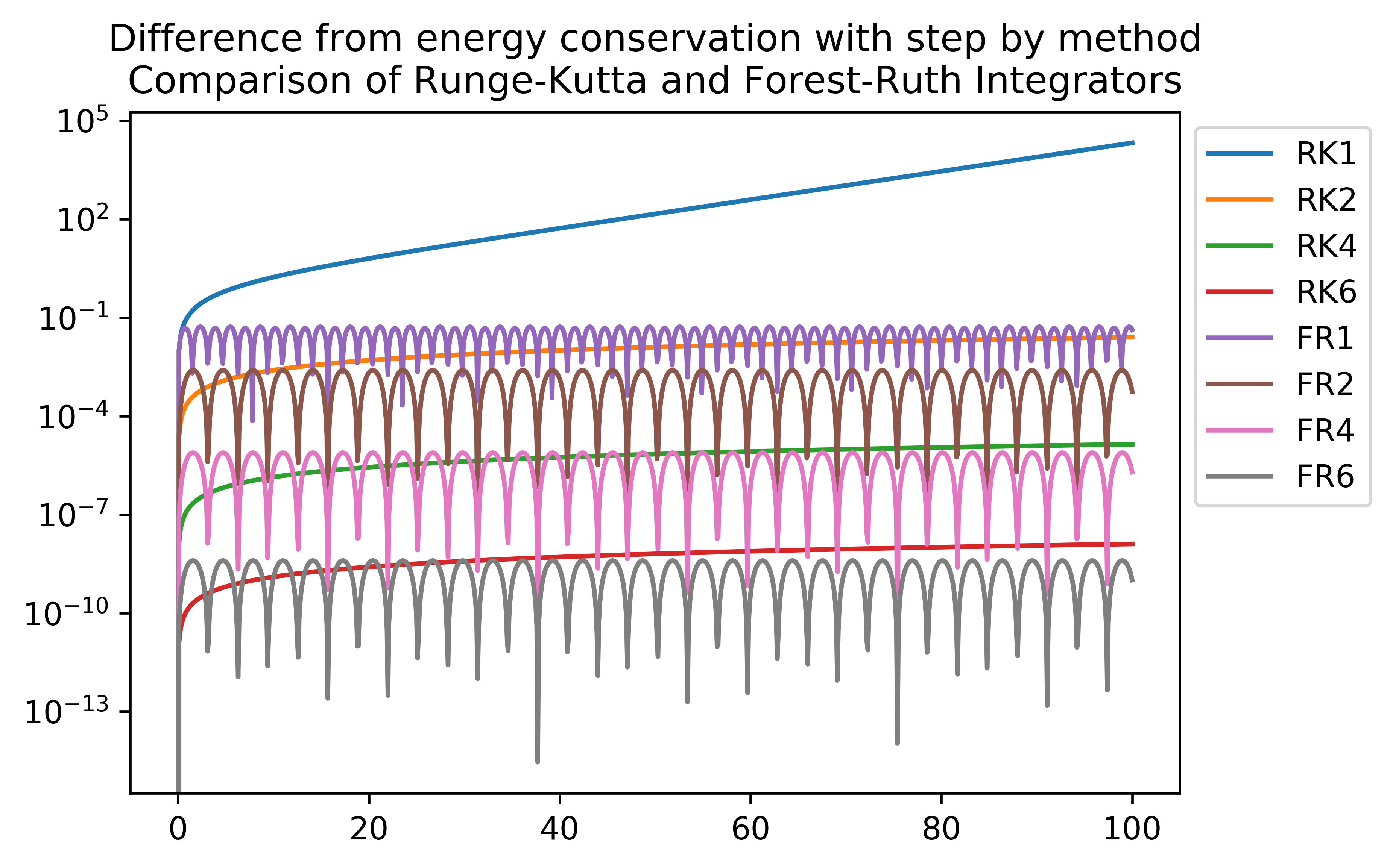
Kepler’s Laws for the orbital motion of two bodies are analytically established relations. Numerical solution methods for these equations of motion may then be compared to the analytic relations. I developed code to numerically solve equations of motion in classical mechanics using a variety of ODE solution methods. The results conserved energy and were in agreement with each of Kepler’s Laws.
ODE Solution Methods:
- Runge Kutta Methods
- Euler (RK1)
- Midpoint (RK2)
- Runge Kutta (RK4)
- Luther’s Sixth Order Method (RK6)
- Symplectic Methods
- Symplectic Euler (FR1)
- Stormer Verlet (FR2)
- Forest Ruth (FR4)
- Yoshida’s Sixth Order Method (FR6)
Here are plots of the numeric verification of Kepler’s Third Law, and energy conservation for each solution method:

Writing brings a degree of permanency to knowledge. The content of computerized writing such as pdfs are easily searched and shared. The factors of permanency, searching, and sharing have motivated my pursuit of scientific typesetting.
My first foray into typesetting was in 2012 when, with the encouragement of Professor Paul Zeitz, I wrote an 8500 word manuscript on geometry, symmetry, and number theory. A few years later, in my thermodynamics/optics/modern physics class with Professor David Everitt, I typeset 238 problems, so that future students could more simply approach the homework. Around this same time I began typesetting formula sheets, some of which you may find here.
During my first year at UCLA, I took a thermodynamics class with Professor Vasilios Manousiouthakis. He began the class by announcing: “I intend for this to be the hardest class you ever take.” It was. Vasilios required us to typeset our homework sets, warranting that: “yes, it is tedious, but you will catch your errors.” I found that typing did catch my errors, and since then, I have typed several hundred pages of homework in LaTeX.
Here is a graphic of projectile motion in a non-inertial reference frame, and an excerpt from a formula sheet on solid state physics:


- Simulation of Chemical Engineering Unit Operations (2018)
- Chemical Engineering Club Group Projects
- ChIP Project, Winter 2018 – Building a Cooling Tower (group lead)
- LEAP Project, Winter 2018 – Modeling Ammonia Production
- LEAP Project, Fall 2017 – Bruin Whiskey (group lead)
- Mechanical Problem Solving
- Electron Beam Evaporator (2018)
- Spectrometers at College of Marin (2016-2017)
- Gas Chromatograph Mass Spectrometer
- Infrared Spectrometer
- Proton NMR Spectrometer
- Development of Chemistry Lab Course Material (2016-2017)
- Materials science paper reviewing FinFET processing techniques, 20 pages (2017)
- Lecture titled “Prostanoids: Synthesis and Function” (2015)